Teoría Atómica III: La dualidad onda-partícula y el electrón
¿Sabías que los átomos no podían describirse con precisión hasta que se desarrolló la teoría cuántica? La teoría cuántica ofreció una nueva forma de pensar sobre el universo a nivel atómico. Después de los enormes avances en mecánica cuántica del siglo pasado, la posición de los electrones y otras partículas infinitesimales se puede predecir con confianza.
As discussed in our Atomic Theory II module, at the end of 1913 Niels Bohr facilitated the leap to a new paradigm of atomic theory – quantum mechanics. Bohr’s new idea that electrons could only be found in specified, quantized orbits was revolutionary (Bohr, 1913). As is consistent with all new scientific discoveries, a fresh way of thinking about the universe at the atomic level would only lead to more questions, the need for additional experimentation and collection of evidence, and the development of expanded theories. As such, at the beginning of the second decade of the 20th century, another rich vein of scientific work was about to be mined.
In the late 19th century, the father of the periodic table, Russian chemist Dmitri Mendeleev, had already determined that the elements could be grouped together in a manner that showed gradual changes in their observed properties. (This is discussed in more detail in our module The Periodic Table of Elements.) By the early 1920s, other periodic trends, such as atomic volume and ionization energy, were also well established.
Figura 1: La tabla periódica de elementos.
The German physicist Wolfgang Pauli made a quantum leap by realizing that in order for there to be differences in ionization energies and atomic volumes among atoms with many electrons, there had to be a way that the electrons were not all placed in the lowest energy levels. If multi-electron atoms did have all of their electrons placed in the lowest energy levels, then very different periodic patterns would have resulted from what was actually observed. However, before we reach Pauli and his work, we need to establish a number of more fundamental ideas.
The development of early quantum theory leaned heavily on the concept of wave-particle duality. This simultaneously simple and complex idea is that light (as well as other particles) has properties that are consistent with both waves and particles. The idea had been first seriously hinted at in relation to light in the late 17th century. Two camps formed over the nature of light: one in favor of light as a particle and one in favor of light as a wave. (See our Light I: Particle or Wave? module for more details.) Although both groups presented effective arguments supported by data, it wasn’t until some two hundred years later that the debate was settled.
Animación Interactiva: Atomic and ionic structure of the first 12 elements
At the end of the 19th century the wave-particle debate continued. James Clerk Maxwell, a Scottish physicist, developed a series of equations that accurately described the behavior of light as an electromagnetic wave, seemingly tipping the debate in favor of waves. However, at the beginning of the 20th century, both Max Planck and Albert Einstein conceived of experiments which demonstrated that light exhibited behavior that was consistent with it being a particle. In fact, they developed theories that suggested that light was a wave-particle – a hybrid of the two properties. By the time of Bohr’s watershed papers, the time was right for the expansion of this new idea of wave–particle duality in the context of quantum theory, and in stepped French physicist Louis de Broglie.
In 1924, de Broglie published his PhD thesis (de Broglie, 1924). He proposed the extension of the wave-particle duality of light to all matter, but in particular to electrons. The starting point for de Broglie was Einstein’s equation that described the dual nature of photons, and he used an analogy, backed up by mathematics, to derive an equation that came to be known as the “de Broglie wavelength” (see Figure 1 for a visual representation of the wavelength).
The de Broglie wavelength equation is, in the grand scheme of things, a profoundly simple one that relates two variables and a constant: momentum, wavelength, and Planck's constant. There was support for de Broglie’s idea since it made theoretical sense, but the very nature of science demands that good ideas be tested and ultimately demonstrated by experiment. Unfortunately, de Broglie did not have any experimental data, so his idea remained unconfirmed for a number of years.
Figura 2: dos representaciones de una longitud de onda de De Broglie (la línea azul) usando un átomo de hidrógeno: una vista radial (A) y una vista 3D (B).
It wasn’t until 1927 that de Broglie’s hypothesis was demonstrated via the Davisson-Germer experiment (Davisson, 1928). In their experiment, Clinton Davisson and Lester Germer fired electrons at a piece of nickel metal and collected data on the diffraction patterns observed (Figure 2). The diffraction pattern of the electrons was entirely consistent with the pattern already measured for X-rays and, since X-rays were known to be electromagnetic radiation (i.e., waves), the experiment confirmed that electrons had a wave component. This confirmation meant that de Broglie’s hypothesis was correct.
Figura 3: un dibujo del experimento realizado por Davisson y Germer en el que dispararon electrones a una pieza de níquel metálico y observaron los patrones de difracción.
image ©Roshan220195Interestingly, it was the (experimental) efforts of others (Davisson and Germer), that led to de Broglie winning the Nobel Prize in Physics in 1929 for his theoretical discovery of the wave-nature of electrons. Without the proof that the Davisson-Germer experiment provided, de Broglie’s 1924 hypothesis would have remained just that – a hypothesis. This sequence of events is a quintessential example of a theory being corroborated by experimental data.
Punto de Comprensión
In 1926, Erwin Schrödinger derived his now famous equation (Schrödinger, 1926). For approximately 200 years prior to Schrödinger’s work, the infinitely simpler F = ma (Newton’s second law) had been used to describe the motion of particles in classical mechanics. With the advent of quantum mechanics, a completely new equation was required to describe the properties of subatomic particles. Since these particles were no longer thought of as classical particles but as particle-waves, Schrödinger’s partial differential equation was the answer. In the simplest terms, just as Newton’s second law describes how the motion of physical objects changes with changing conditions, the Schrödinger equation describes how the wave function (Ψ) of a quantum system changes over time (Equation 1). The Schrödinger equation was found to be consistent with the description of the electron as a wave, and to correctly predict the parameters of the energy levels of the hydrogen atom that Bohr had proposed.
Equation 1: The Schrödinger equation.
Schrödinger’s equation is perhaps most commonly used to define a three-dimensional area of space where a given electron is most likely to be found. Each area of space is known as an atomic orbital and is characterized by a set of three quantum numbers. These numbers represent values that describe the coordinates of the atomic orbital: including its size (n, the principal quantum number), shape (l, the angular or azimuthal quantum number), and orientation in space (m, the magnetic quantum number). There is also a fourth quantum number that is exclusive to a particular electron rather than a particular orbital (s, the spin quantum number; see below for more information).
Schrödinger’s equation allows the calculation of each of these three quantum numbers. This equation was a critical piece in the quantum mechanics puzzle, since it brought quantum theory into sharp focus via what amounted to a mathematical demonstration of Bohr’s fundamental quantum idea. The Schrödinger wave equation is important since it bridges the gap between classical Newtonian physics (which breaks down at the atomic level) and quantum mechanics.
The Schrödinger equation is rightfully considered to be a monumental contribution to the advancement and understanding of quantum theory, but there are three additional considerations, detailed below, that must also be understood. Without these, we would have an incomplete picture of our non-relativistic understanding of electrons in atoms.
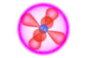
German mathematician and physicist Max Born made a very specific and crucially important contribution to quantum mechanics relating to the Schrödinger equation. Born took the wave functions that Schrödinger produced, and said that the solutions to the equation could be interpreted as three-dimensional probability “maps” of where an electron may most likely be found around an atom (Born, 1926). These maps have come to be known as the s, p, d, and f orbitals (Figure 3).
Figura 4: Basado en las teorías de Born, estas son representaciones de las probabilidades tridimensionales de la ubicación de un electrón alrededor de un átomo. Los cuatro orbitales, en complejidad creciente, son: s, p, d, y f. Se proporciona información adicional sobre el número cuántico magnético del orbital (m).
image ©UC Davis/ChemWikiIn the year following the publication of Schrödinger’s work, the German physicist Werner Heisenberg published a paper that outlined his uncertainty principle (Heisenberg, 1927). He realized that there were limitations on the extent to which the momentum of an electron and its position could be described. The Heisenberg Uncertainty Principle places a limit on the accuracy of simultaneously knowing the position and momentum of a particle: As the certainty of one increases, then the uncertainty of other also increases.
The crucial thing about the uncertainty principle is that it fits with the quantum mechanical model in which electrons are not found in very specific, planetary-like orbits – the original Bohr model – and it also dovetails with Born’s probability maps. The two contributions (Born and Heisenberg’s) taken together with the solution to the Schrödinger equation, reveal that the position of the electron in an atom can only be accurately predicted in a statistical way. That is to say, we know where the electron is most likely to be found in the atom, but we can never be absolutely sure of its exact position.
Punto de Comprensión
In 1922 German physicists Otto Stern, an assistant of Born’s, and Walther Gerlach conducted an experiment in which they passed silver atoms through a magnetic field and observed the deflection pattern. In simple terms, the results yielded two distinct possibilities related to the single, 5s valence electron in each atom. This was an unexpected observation, and implied that a single electron could take on two, very distinct states. At the time, nobody could explain the phenomena that the experiment had demonstrated, and it took a number of scientists, working both independently and in unison with earlier experimental observations, to work it out over a period of several years.
In the early 1920s, Bohr’s quantum model and various spectra that had been produced could be adequately described by the use of only three quantum numbers. However, there were experimental observations that could not be explained via only three mathematical parameters. In particular, as far back as 1896, the Dutch physicist Pieter Zeeman noted that the single valence electron present in the sodium atom could yield two different spectral lines in the presence of a magnetic field. This same phenomenon was observed with other atoms with odd numbers of valence electrons. These observations were problematic since they failed to fit the working model.
In 1925, Dutch physicist George Uhlenbeck and his graduate student Samuel Goudsmit proposed that these odd observations could be explained if electrons possessed angular momentum, a concept that Wolfgang Pauli later called “spin.” As a result, the existence of a fourth quantum number was revealed, one that was independent of the orbital in which the electron resides, but unique to an individual electron.
By considering spin, the observations by Stern and Gerlach made sense. If an electron could be thought of as a rotating, electrically-charged body, it would create its own magnetic moment. If the electron had two different orientations (one right-handed and one left-handed), it would produce two different ‘spins,’ and these two different states would explain the anomalous behavior noted by Zeeman. This observation meant that there was a need for a fourth quantum number, ultimately known as the “spin quantum number,” to fully describe electrons. Later it was determined that the spin number was indeed needed, but for a different reason – either way, a fourth quantum number was required.
Punto de Comprensión
In 1922, Niels Bohr visited his colleague Wolfgang Pauli at Göttingen where he was working. At the time, Bohr was still wrestling with the idea that there was something important about the number of electrons that were found in ‘closed shells’ (shells that had been filled).
In his own later account (1946), Pauli describes how building upon Bohr’s ideas and drawing inspiration from others’ work, he proposed the idea that only two electrons (with opposite spins) should be allowed in any one quantum state. He called this ‘two-valuedness’ – a somewhat inelegant translation of the German zweideutigkeit (Pauli, 1925). The consequence was that once a pair of electrons occupies a low energy quantum state (orbitals), any subsequent electrons would have to enter higher energy quantum states, also restricted to pairs at each level.
Using this idea, Bohr and Pauli were able to construct models of all of the electronic structures of the atoms from hydrogen to uranium, and they found that their predicted electronic structures matched the periodic trends that were known to exist from the periodic table – theory met experimental evidence once again.
Pauli ultimately formed what came to be known as the exclusion principle (1925), which used a fourth quantum number (introduced by others) to distinguish between the two electrons that make up the maximum number of electrons that could be in any given quantum level. In its simplest form, the Pauli exclusion principle states that no two electrons in an atom can have the same set of four quantum numbers. The first three quantum numbers for any two electrons can be the same (which places them in the same orbital), but the fourth number must be either +½ or -½, i.e., they must have different ‘spins’ (Figure 4). This is what Uhlenbeck and Goudsmit’s research suggested, following Pauli’s original publication of his theories.
Figure 5: A model of the fourth quantum number, spin (s). Shown here are models for particles with spin (s) of ½, or half angular momentum.
The period described here was rich in the development of the quantum theory of atomic structure. Literally dozens of individuals, some mentioned throughout this module and others not, contributed to this process by providing theoretical insights or experimental results that helped shape our understanding of the atom. Many of the individuals worked in the same laboratories, collaborated together, or communicated with one another during the period, allowing the rapid transfer of ideas and refinements that would shape modern physics. All these contributions can certainly been seen as an incremental building process, where one idea leads to the next, each adding to the refinement of thinking and understanding, and advancing the science of the field.